Metadata and Queries
This notebok covers accessing and using metadata (data about the data) and basic queries useful when reading geoJSON files from open data sources.
The sodapy module is used to explore metatdata from Socrata based open data sources. You need to install Sodapy using pip in a terminal window.

SODAPY has a method to get_metadata which returns dictionary containing information summarizing the dataset. If you are working with Socrata datasets, it is best to request an application token.

You must create a user name and password login before requesting an APP TOKEN.
With respect to queries, two appraoches are demonstrated, namely using the SODAPY get method and using the geopandas read_file method. Both appraoches use a string containing the url of the SODA endpoint. The query string structure is a bit different and the SODA get method returns a dictionary that has to be converted to a GeoDataFrame.
# import libraries

import sodapy
from sodapy import Socrata

import pandas as pd
import geopandas as gpd
import numpy as np
import os

import matplotlib.pyplot as plt
# draw maps in the notebook
%matplotlib inline
Get polygons that represent neighborhoods in Buffalo, NY.
Find the dataset identifier from the Buffalo Open data website.
Copy from view data window - EXPORT/SODA API - or home page API button.
- Neighborhoods in Buffalo - https://data.buffalony.gov/resource/g7bi-nz8b.json.
- This is a polygon dataset with the boundaries of Buffalo's neighborhoods as defined by the city planning department.
First look at the metadata.
- In this example the field names for each column in the dataset are displayed
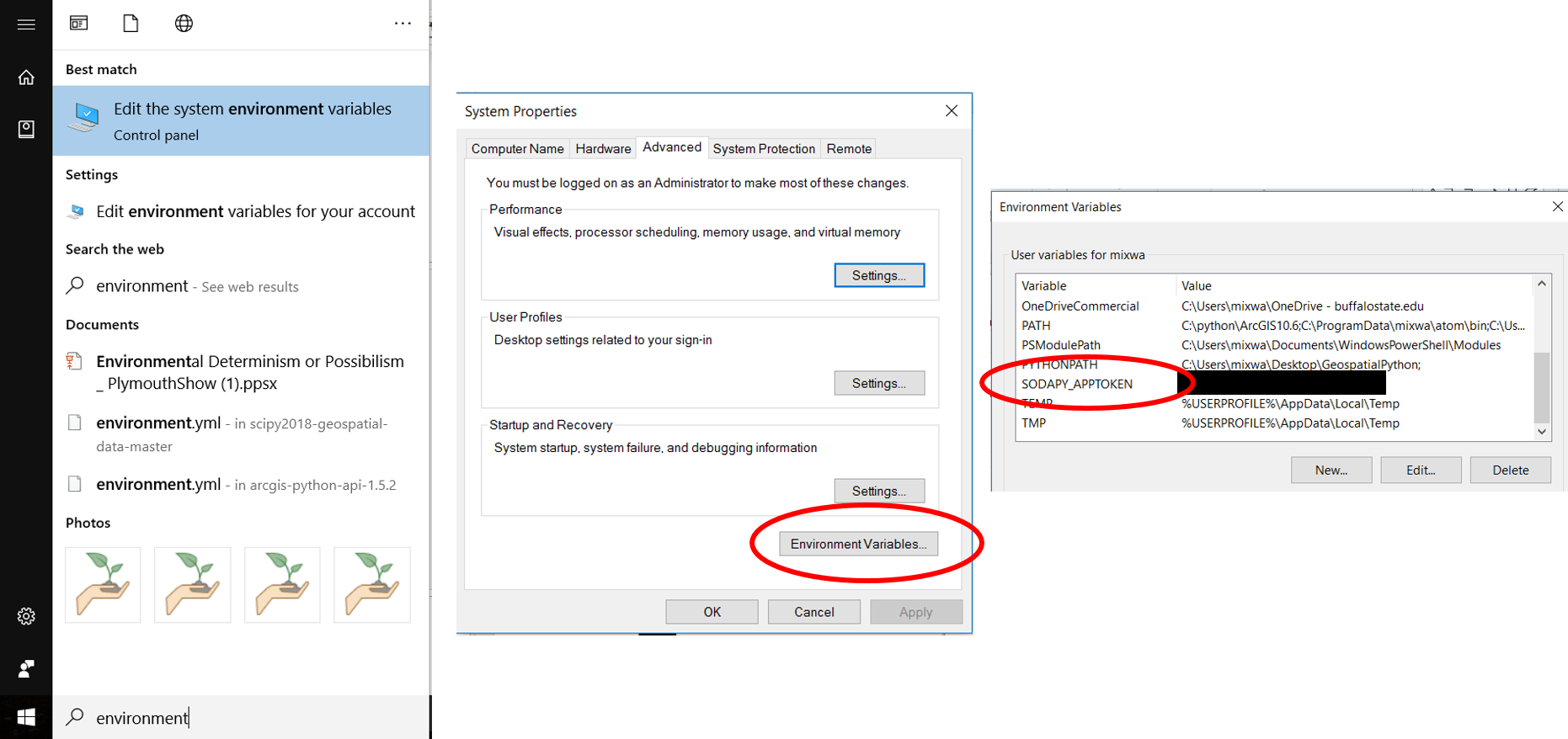
I have stored my SODAPY App Token in my environment variables. In Windows, edit your environment variables. I do not know how to do this on a mac!

If you do not want to modify the environment, you can include your app token as a string but everyone who sees your notebook will see your app token.
socrata_domain = "data.buffalony.gov/"
socrata_dataset_identifier = "g7bi-nz8b"
app_token = os.environ.get("SODAPY_APPTOKEN") # this is in my environment path

client = Socrata(socrata_domain, app_token)
metadata = client.get_metadata(socrata_dataset_identifier)

[x['fieldName'] for x in metadata['columns']]# show field names in dataset
View metadata for specific fields
You can view the metadata for each field to find out
- the data type,
- how many null values there are, and
- get a frequency distribution of the top values if relevant.
meta_geom = [x for x in metadata['columns'] if x['fieldName'] == 'the_geom'][0]
meta_geom
meta_name = [x for x in metadata['columns'] if x['fieldName'] == 'nbhdname'][0]
meta_name
Use SODAPY GET
- To read the entire data set
- To read one neighborhood
You must include content_type ='geojson'. The result is a dictionary.
allNeigh = client.get(socrata_dataset_identifier,content_type='geojson')
#allNeigh
ElmBid = client.get(socrata_dataset_identifier,content_type='geojson',nbhdname = 'Elmwood Bidwell')
#ElmBid
Convert dictionary to geoDataFrame from features
nbhood=gpd.GeoDataFrame.from_features(allNeigh)
nbhood.plot();
elmBid=gpd.GeoDataFrame.from_features(ElmBid)
elmBid.plot();
Alternatively
Use geopandas.read_file with the url to get the geojson version of the file.
To only read a single neightborhood, add ?$where=nbhdname=\%27Elmwood\%20Bidwell\%27 to the url
url1="https://data.buffalony.gov/resource/g7bi-nz8b.geojson"

#If no SODA API
# url = "https://data.buffalony.gov/api/geospatial/q9bk-zu3p?method=export&format=GeoJSON"

gdf = gpd.read_file(url1)
Read only 1 neighborhood
In a where clause you have to specify the url encode values. %27= ' and %20 = space
url2="https://data.buffalony.gov/resource/g7bi-nz8b.GeoJSON?$where=nbhdname=%27Elmwood%20Bidwell%27"
ngdf = gpd.read_file(url2)
gdf.plot();
ngdf.plot();
If the coordinate reference system is not projected, change to EPSG:3857 and plot the file using matplotlib. Colors are based on the neighborhood name field.
gdf.shape
gdf.geometry.name #renamed the_geom to geometry
gdf.crs
EPSG 4326 is WGS 84, units = degrees (unprojected)
Reproject to EPSG 3857 is Web Mercator Auxiliary Sphere, WGS 84, units = meters
gdf=gdf.to_crs('epsg:3857')
gdf.plot(column='nbhdname', figsize=(9,10));
Create a new dataframe and with a new field containing sq. kilometers.
The data owner provided a field with sq. miles and acres calculated. We could use either (or both) of these for a choropleth map. But, since the new units of the projected data is meters, we can calculate sq. kilometers as a third measure of size for a choropleth map.
neighborhoods = gdf[['nbhdname', 'geometry', 'sqmiles']].copy()
neighborhoods['sqkilo']=neighborhoods.geometry.area/1000**2 # in sq kilometers
neighborhoods.nbhdname+ ' Area = '+neighborhoods.sqkilo.astype(str)
Get open data on pot hole service requests
The City of Buffalo has an open data set on 311 request for service calls. One type of call they receive from the public is for pot hole repair. On Feb 16, WIVB reported on the city's pot hole blitz (https://www.wivb.com/news/local-news/city-of-buffalo-goes-on-saturday-pothole-blitz/1788423791). The story indicted where the crews were dispatched to fix the pot holes.
The blitz included:
2 crews on Main Street between Humboldt and Hertel
1 crew on South Park Avenue between Bailey and Dorrance
1 crew the Hamlin Park neighborhood
1 crew the Broadway Fillmore area
4 other crews across the city on various pothole requests that were logged into 311.
The story went on to indicate:
"The City of Buffalo said that 311 calls are not as high as they were in 2018. In February 2018, the city got 1,100 calls for pot hole repair through 311. In the two weeks of February 2019, the city said there have been 400 calls."
We will pull data for the first two weeks in Feb 2019 and map that data to the Buffalo Neighborhoods. The SODA endpoint is:
311 Service Requests https://data.buffalony.gov/resource/whkc-e5vr.geojson
Two methods are shown to query the data:
- using SODAPY
- using geopandas read_file
There are three commonly used parameters in a query:
- \$limit - to increase the number of records beyond the default of 1,000
- \$where - read specific rows (records)
\$select - read specific columns (fields)
See the API Docs (Developers) for a full list of parameters (SQLQueries) https://dev.socrata.com/docs/queries/
Read data into a geodataframe since there is geometry in the dataset. The query will include
- type contains 'Pot Hole" and open_date between 2/1/2019 and 2/15/2019.
socrata_dataset_identifier = "whkc-e5vr"
metadata = client.get_metadata(socrata_dataset_identifier)
[x['fieldName'] for x in metadata['columns']]# show field names in dataset
ph_2019 = client.get(socrata_dataset_identifier,
                     content_type='geojson',
                     where ="(open_date between '2019-02-01T00:00:00' AND '2019-02-15T00:00:00') AND (type like 'Pot Hole%')")

phgdf = gpd.GeoDataFrame.from_features(ph_2019)
phgdf.shape
Geopandas URL
is a bit more complicated than the sodapy one since there is no client to convert the url to the proper codes. The only new code in this url is %25 which is the code for % which is the wild card character for searching substrings, Basically, this will read any row between the appropriate dates and whre the type field contains "Pot Hole%". The string must start with the Pot and Hole can be followed by any number of characters.
url3='https://data.buffalony.gov/resource/p7e8-krif.geojson?\
$where=open_date%20between%20%272019-02-01T00:00:00%27%20and%20%272019-02-15T00:00:00%27\
%20and%20type%20like%20%27Pot%20Hole%25%27'

phgdf2 =  gpd.read_file(url3)
phgdf2.shape
Just for fun, read the 2020 calls for Pot Hole repairs during the first two weeks of February.
url4='https://data.buffalony.gov/resource/p7e8-krif.geojson?$limit=1000000&\
$where=open_date%20between%20%272020-02-01T00:00:00%27%20and%20%272020-02-15T00:00:00%27\
%20and%20type%20like%20%27Pot%20Hole%25%27'

phgdf3 =  gpd.read_file(url4)
phgdf3.shape
phgdf2.tail()
phgdf2['council_district'] = phgdf2.council_district.fillna("UNKNOWN")
phgdf2=phgdf2.loc[phgdf2.geometry.notnull()]
phgdf2=phgdf2.to_crs('epsg:3857')
phgdf2.plot(column='council_district',figsize=(9,10),legend=True);
It appears that the UNKNOWN Council District should actually = NORTH. Change UNKNOWN to NORTH.
phgdf2['council_district'].replace({"UNKNOWN":"NORTH"}, inplace=True)
phgdf2.plot(column='council_district',figsize=(9,10),legend=True);
Another query example.
Find all pot hole complaints within a mile of my house.
- Need the coordinates of my house (lat/lon) which is (y,x)
- Converision of a mile to meters
- within_circle(location,42.915431,-78.877030,1609)
- Instead of reading all columns, use \$select to keep a few of them
- Extract the year and month from open_date
- date_extract_y(open_date)%20as%20year,date_extract_m(open_date)%20as%20month
url="https://data.buffalony.gov/resource/p7e8-krif.geojson?$limit=10000&\
$select=date_extract_y(open_date)%20as%20year,date_extract_m(open_date)%20as%20month,subject,reason,type,location&\
$where=within_circle(location,42.915431,-78.877030,1609)\
%20and%20type%20like%20%27Pot%20Hole%25%27"
phnear = gpd.read_file(url)

phnear.tail()
phnear=phnear.to_crs('epsg:3857')
phnear.plot(column='year',figsize=(9,9), legend=True);
phsummary=phnear.groupby(['year','month']).agg({'month':'count'})
phsummary.columns = ['Count_Mth']
phsummary=phsummary.reset_index()
phsummary
phsummary.loc[phsummary['Count_Mth'].idxmax()]
Assignment: New York City 311 data analysis
Borough Boundaries (water areas excluded) https://data.cityofnewyork.us/resource/7t3b-ywvw.geojson
311 Service Requests from 2010 to present https://data.cityofnewyork.us/resource/erm2-nwe9.geojson
where:
- created_date between 1/1/2018 and 3/1/2020
- descriptor contains Loud Music select:
- keep year and month of created_date
- keep - city, borough, location, open_data_channel_type, complaint_type, descriptor
Answer the following questions:
- Which Borough had the most noise complaints during this time period?
- During what month are noise complaints most frequent?
- How many compaints by borough are from residential propoerties versus commercial?
- What channel type is most frequently used, by borrough.
Map all commercial complaints (use the borough boundaries as the back drop behind the points.)
Let's make prettier maps. Below is an example that leads to adding a basemap, polygons, and points to the same map plot!
ax = gdf.plot(figsize=(10, 10), alpha=0.5, edgecolor='k') # plots polygons
# conda install -c conda-forge contextily
import contextily as ctx
ax = gdf.plot(figsize=(10, 10), alpha=0.5, edgecolor='k')
ctx.add_basemap(ax) # add default basemap to plot
ax = gdf.plot(figsize=(10, 10), alpha=0.5, edgecolor='k')
ctx.add_basemap(ax, url=ctx.providers.Stamen.TonerLite) #change basemap from ctx.providers
nei = gdf.plot(figsize=(10, 10), alpha=0.5, edgecolor='k')
ctx.add_basemap(nei, url=ctx.providers.Stamen.TonerLite)
phgdf2.plot(ax=nei, marker='o', color='red', markersize=5);#add points to plot